Material Inelasticity
Distributed inelasticity elements are becoming widely employed in earthquake engineering applications, either for research or professional engineering purposes. Whilst their advantages in relation to the simpler lumped-plasticity models, together with a concise description of their historical evolution and discussion of existing limitations, can be found in e.g. Filippou and Fenves [2004] or Fragiadakis and Papadrakakis [2008], here it is simply noted that distributed inelasticity elements do not require (not necessarily straightforward) calibration of empirical response parameters against the response of an actual or ideal frame element under idealized loading conditions, as is instead needed for concentrated-plasticity phenomenological models.
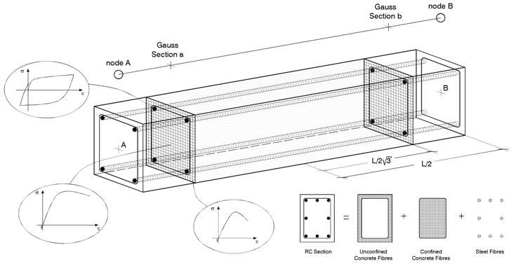
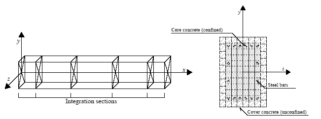
In SeismoStruct, use is made of the so-called fibre approach to represent the cross-section behaviour, where each fibre is associated with a uniaxial stress-strain relationship; the sectional stress-strain state of beam-column elements is then obtained through the integration of the nonlinear uniaxial stress-strain response of the individual fibres (typically 100-150) in which the section has been subdivided (the discretisation of a typical reinforced concrete cross-section is depicted, as an example, in the figure below).
Such models feature additional assets, which can be summarized as: no requirement of a prior moment-curvature analysis of members; no need to introduce any element hysteretic response (as it is implicitly defined by the material constitutive models); direct modelling of axial load-bending moment interaction (both on strength and stiffness); straightforward representation of biaxial loading, and interaction between flexural strength in orthogonal directions.
Distributed inelasticity frame elements can be implemented with two different finite elements (FE) formulations: the classical displacement-based (DB) ones [e.g. Hellesland and Scordelis 1981; Mari and Scordelis 1984], and the more recent force-based (FB) formulations [e.g. Spacone et al. 1996; Neuenhofer and Filippou 1997]. In a DB approach the displacement field is imposed, whilst in a FB element equilibrium is strictly satisfied and no restraints are placed to the development of inelastic deformations throughout the member; see e.g. Alemdar and White [2005] and Freitas et al. [1999] for further discussion.
In the DB case, displacement shape functions are used, corresponding for instance to a linear variation of curvature along the element. In contrast, in a FB approach, a linear moment variation is imposed, i.e. the dual of previously referred linear variation of curvature. For linear elastic material behaviour, the two approaches obviously produce the same results, provided that only nodal forces act on the element. On the contrary, in case of material inelasticity, imposing a displacement field does not enable to capture the real deformed shape since the curvature field can be, in a general case, highly nonlinear. In this situation, with a DB formulation a refined discretisation (meshing) of the structural element (typically 4-5 elements per structural member) is required for the computation of nodal forces/displacements, in order to accept the assumption of a linear curvature field inside each of the sub-domains. Still, in the latter case users are not advised to rely on the values of computed sectional curvatures and individual fibre stress-strain states.
Instead, a FB formulation is always exact, since it does not depend on the assumed sectional constitutive behaviour. In fact, it does not restrain in any way the displacement field of the element. In this sense this formulation can be regarded as always "exact", the only approximation being introduced by the discrete number of the controlling sections along the element that are used for the numerical integration. A minimum number of 3 Gauss-Lobatto integration sections are required to avoid under-integration, however such option will in general not simulate the spread of inelasticity in an acceptable way. Consequently, the suggested minimum number of integration points is 4, although 5-7 IPs are typically used (see figure below). Such feature enables to model each structural member with a single FE element, therefore allowing a one-to-one correspondence between structural members (beams and columns) and model elements. In other words, no meshing is theoretically required within each element, even if the cross section is not constant. This is because the force field is always exact, regardless of the level of inelasticity.
In SeismoStruct, both aforementioned DB and FB element formulations are implemented, with the latter being typically recommended, since, as mentioned above, it does not in general call for element discretisation, thus leading to considerably smaller models, with respect to when DB elements are used, and thus much faster analyses, notwithstanding the heavier element equilibrium calculations. An exception to this non-discretisation rule arises when localisation issues are expected, in which case special cautions/measures are needed, as discussed in Calabrese et al. [2010].
In addition, the use of a single element per structural element gives users the possibility of readily employing element chord-rotations output for seismic code verifications (e.g. Eurocode 8, FEMA-356, ATC-40, etc). Instead, when the structural member has had to be discretised in two or more frame elements (necessarily the case for DB elements), then users need to post-process nodal displacements/rotation in order to estimate the members chord-rotations [e.g. Mpampatsikos et al. 2008].
Finally, it is noted that, for reasons of higher accuracy, the Gauss quadrature is employed in those cases where two or three integration sections are chosen by the user (it is recalled that for DB elements only the former is possible), whilst Lobatto quadrature is used in those cases where four to ten integration sections are defined. Although users may and should refer to the literature (or to this online resource) for further details on such rules, the approximate coordinates along the element's length (measured from its baricentre) of the integration sections is given below:
- 2 integration sections: [-0.577 0.577] x L/2
- 3 integration sections: [-1 0.0 1] x L/2
- 4 integration sections: [-1 -0.447 0.447 1] x L/2
- 5 integration sections: [-1 -0.655 0.0 0.655 1] x L/2
- 6 integration sections: [-1 -0.765 -0.285 0.285 0.765 1] x L/2
- 7 integration sections: [-1 -0.830 -0.469 0.0 0.469 0.830 1] x L/2
- 8 integration sections: [-1 -0.872 -0.592 -0.209 0.209 0.592 0.872 1] x L/2
- 9 integration sections: [-1 -0.900 -0.677 -0.363 0.0 0.363 0.677 0.900 1] x L/2
- 10 integration sections: [-1 -0.920 -0.739 -0.478 -0.165 0.165 0.478 0.739 0.920 1] x L/2
Notes
- It is immediate with FB formulations to take into account loads acting along the member, while this is not the case for DB approaches, where distributed loads need to be transformed into equivalent point forces/moments at the end nodes of the element (and then lengthy stress-recovery need to be employed to retrieve accurate member action-effects).
- Should the user wish to, it is possible to adopt a concentrated plasticity approach employing the inelastic displacement-based plastic-hinge element (infrmDBPH), as opposed to the distributed inelasticity modelling philosophy intrinsic to the other beam-column elements of SeismoStruct - for instance the inelastic force-based plastic hinge frame element (infrmFBPH) also concentrates the inelasticity at the two ends of the element, however within a fixed length of the element. The same modelling effect can be achieved by making use of the elastic beam-column frame element (elfrm) coupled with nonlinear links placed at its end-nodes. Such modelling approach should however be used with care, since accuracy of the analysis may be compromised whenever users are not highly experienced in the calibration of the available response curves, used in the definition of link elements, the uncoupled DOFs nature of which does also not permit the modelling of the necessary moment-axial force interaction curves/surfaces.
- As mentioned above, the distributed inelasticity modelling, on the other hand, requires no modelling experience since all that is required from the user is to introduce the geometrical and material characteristics of structural members (i.e. engineering parameters). Its use is therefore highly recommended and will grant an accurate prediction of the nonlinear response of structures.
- Users are also invited to read the NEHRP Seismic Design Technical Brief No. 4, in which the nonlinear modelling is well covered.