Processor

Depending on the size of the structure, the selected frame elements type, the applied loads and the processing capacity of the computer being used, the analysis may last some seconds (static analysis), several minutes (time-history analysis) or even hours (time-history analysis of large complex 3D models).

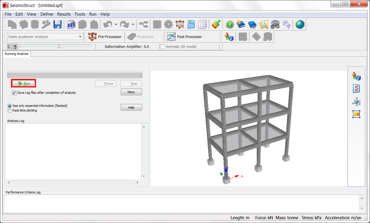
As the analysis is running, a progress bar provides the user with a percentage indication of how far has the former advanced to. Users can in this manner quickly assess the waiting time required for the analysis to be completed, and hence quickly plan their subsequent work schedule. The analysis can also be paused, enabling users to (i) momentarily free computing resources so as to carry out an urgent priority task or (ii) check the results obtained up to that point, which may be useful to decide the worthiness of progressing with a lengthy analysis. If the user presses the Run button again, the analysis can be continued.

The Analysis Log is also shown to the user, in real-time, providing expedient information on the progress of the analysis, loading control and convergence conditions (for each global load increment). This log is saved on a text file (*.log) that features the same name as the project file and which indicates the date and time of when the analysis was run (the sort of non-technical information that comes very handy on occasions). In addition, if the user has specified code-based checks or performance criteria to be checked during the analysis, then the corresponding real-time log is also shown during the analysis and saved to the same *.log file.

At the bottom of the window, the convergence norms at the end of a given (global) load increment are shown. It is noted that, as in the case of the Analysis Log described above, this information does not refer to local load increment/iterations of force-based elements mentioned here.

Finally, the user has also the option of graphically observing the real-time plotting of a capacity (static pushover) or displacement time-history (time-history analysis) curve of any given node and respective degree-of-freedom, pre-selected in the Output module. This option, however, might slow down the analysis and increase its running time when used in relatively slow computers, for which reason the user has also the possibility of simply disabling any real-time plotting, choosing to follow only the analysis logs. Furthermore, displaying of the latter can also be disabled (pressing the Less button) so as to attain even faster performance (on modern fast computers, however, the difference should be completely negligible).

Notes

1. Upon start of the analysis, users may be presented with a warning message regarding 'Zero diagonal terms encountered in a give node'. This means that such node is unrestrained in the degrees-of-freedom indicated (i.e. the node is not connected to an element or constraint capable of providing any restrain/stiffness in such dofs), a condition that, if unintended, implies the presence of an error in the assemblage of model. If, instead, such unrestrained nodal dofs have been intentionally introduced, the user may proceed with the analysis, knowing however that numerical convergence difficulties may arise more easily in such cases.
2. When running an eigenvalue analysis, user may be presented with a message stating: "could not re-orthogonalise all Lanczos vectors", meaning that the Lanczos algorithm, currently the eigenvalue solver in SeismoStruct, could not calculate all or some of the vibration modes of the structure. This behaviour may be observed in either (i) models with assemblage errors (e.g. unconnected nodes/elements) or (ii) complex structural models that feature links/hinges etc. If users have checked carefully their model and found no modelling errors, then they may perhaps try to "simplify" it, by removing its more complex features until the attainment of the eigenvalue solutions. This will enable a better understanding of what might be causing the analysis problems, and thus assist users in deciding on how to proceed. This message typically appears when too many modes are sought, e.g. when 30 modes are asked in a 24 DOF model, or when the eigensolver cannot simply find so many modes (even if DOFs > modes).
3. It is noted that the current version of SeismoStruct does not feature multi-threading capabilities, that is, is not capable of taking advantage of multi-processor computing hardware, hence speed of a single analysis may be increased only by increasing the CPU speed (together with the speeds of the CPU Cache, the Front Side Bus, the RAM modules, the Video RAM, the Hard-Disk (rotation and access)). Having more than one CPU, however, will reduce running times of multiple contemporary analyses, since in such cases "parallel processing" can take place. It is also noted that, currently, SeismoStruct cannot make use of more than 2GB of memory for a given analysis, hence again, having larger memory capacity will be advantageous only when multiple analyses are to be run in simultaneous.
4. There is a size limitation of the output file in SeismoStruct (4GB in 64-bit Windows systems and 3GB in 32-bit Windows systems)
5. Up until now, the development of SeismoStruct has focused primarily on the achievement of ease-of-use and high technical capabilities, with an obvious sacrifice in terms of speed of analysis, something that we hope to address in the future. In the meantime, however, please make sure that your model does not feature an unnecessarily excessive number of elements, section fibres, load increments or iterations, all of which, together with too-stringent convergence criteria, contribute to slow analyses.
6. When using the less numerically stable Frontal solver, it may happen that analysis stop for no apparent reason, at different time-steps. On such occasions, users are advised to change to the default Skyline solver.