Shallow footings macro-element - ssilink1
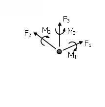
This element is a nonlinear macro-element model for soil-structure interaction of shallow foundations based on the work of Correia and Paolucci [2019]. This macro-element approach reduces the size of the problem significantly, since the footing and the soil are considered as a single macro-element characterized by six degrees-of freedom (6 DOFs), in the 3D case, whose formulation is based on the resultant forces and displacements. The geometry considered herein corresponds to a rectangular rigid footing, with coupling between all the macro-element DOFs and its definition as a single zero-length link element. Considering a planar loading, for simplicity of notation and visualisation, the footing will be subjected to a rocking moment and to both vertical and horizontal forces (My, N and Hx respectively) as evident in the Figure below.
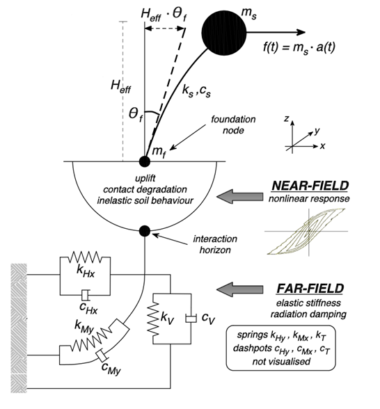
An uplift model is adopted which is based on a nonlinear elastic-uplift response which also considers some degradation of the contact at the soil/footing interface due to irrecoverable changes in its geometry. A bounding surface plasticity model is also used which correctly takes into account the simultaneous elastic-uplift and plastic nonlinear responses. Finally, this macro-element formulation is fully applicable to three-dimensional loading cases. The above are schematically illustrated in the Figure below.
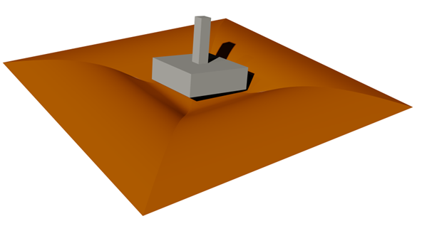
The footing macro-element model represents the dynamic behaviour of isolated rigid footings, subjected to three-dimensional inertial loading, from the initial stages of loading up until reaching failure. The macro-element is based on the three major features of the response of footings, namely:
i) Initial elastic response,
ii) Uplift in rocking response,
iii) Failure loading conditions.
The bounding surface plasticity model is used to represent a continuous transition between the initial elastic response and the plastic flow at failure, for monotonic, cyclic and dynamic loading conditions. The uplift phenomenon is represented by a nonlinear elastic model which, however, takes into account and is influenced by the plastic deformation state in the underlying soil.
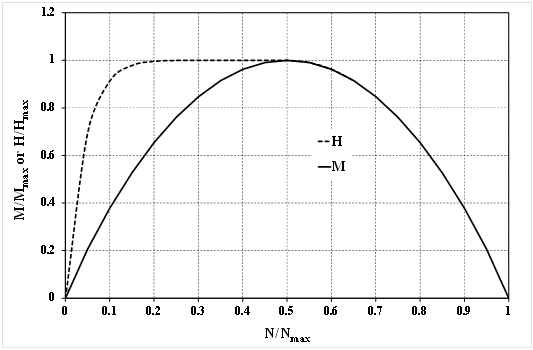
The bounding surface adopted in this macro-element depends on the type of soil and its drainage conditions during a seismic event. Therefore, different 3D failure surfaces are considered for drained and undrained conditions. The ultimate surface adopted to describe the drained behaviour corresponds to the “rugby-ball” shape, while for undrained loading the ultimate surface corresponds to the so-called "scallop" shape, which is represented in the Figure below in terms of its intersection in the H-N and M-N planes of loading. The "rugby-ball" shape corresponds to have the ultimate surface represented by the continuous line in both planes of loading.
Twenty five parameters are required for the definition of the macro-element model from which only three need to be calibrated:
- The footing dimensions (length, L, and width, B).
- The six foundation initial stiffness components for vertical, horizontal and rotational directions (KN1, KH2, KH3, KM2, KM3, KM2, KTT) which can be evaluated by using formulas from literature [e.g. Gazetas, 1991], or calibrated based on test results. The same applies to the corresponding six equivalent dashpot coefficients for radiation damping representation.
- the maximum centred vertical load capacity Nmax that corresponds to the ultimate static bearing capacity of the foundation and can be evaluated by standard superposition formulas [e.g. Brinch-Hansen,1970]
- the maximum base shear capacities Hmax2 and Hmax3 and maximum base moment capacities Mmax2, Mmax3, Tmax, which can be calibrated based either on material properties (e.g. soil friction angle) or on theoretical values [Butterfield and Gottardi, 1994]
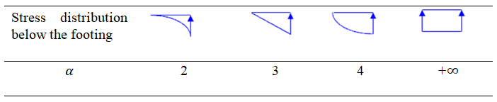
- the uplift initiation parameter, α, is only dependent on the assumed stress distribution of vertical stresses underneath the foundation as illustrated in the Figure below and can be determined from simple static considerations. It is not affecting much the results, and is typically taken as 3, which corresponds to assuming a linear distribution stresses for the soil at the beginning of the analysis
- the exponent for loading history in unloading/reloading, nUR, is usually equal to 1, being related to different plastic modulus values for unloading/reloading in comparison to the virgin loading
- the soil/footing contact degradation parameter,
 , takes into account the decrease of the contact area due to cumulative inelastic rocking in the damage model and can be evaluated based on experimental results
 - the normalised reference plastic modulus,H0pl calibrated based on experimental results
- the plastic potential surface parameter,
 , also calibrated based on experimental results
From the above, it turns out that, once the classical elastic and strength parameters for the soil- foundation system are known, a small number of 3 free-parameters remains to be calibrated in the validation process: , the normalised reference plastic modulus, ![]() the plastic potential surface parameter, and
the plastic potential surface parameter, and ![]() , the damage model parameter.
, the damage model parameter.
Notes
- Given that the SSI macro-element presents a nonlinear response from the outset of the analysis, it is very important to apply the initial loading in several steps in order to avoid lack of convergence or erroneous results. Typically a number of steps between 50 and 100 should be enough, although in more demanding cases of analyses might be needed.
- Care should be taken on the ground motion input when a dynamic time history analysis with the SSI macro-element is made. In fact, given that the two nodes of the macro-element should have the same motion while no inertial interaction is present, the soundest way of performing the analysis is not by imposing the ground motion acceleration history at the base node but by imposing the corresponding inertia forces on the structural masses above.
Some theoretical background on SSI analysis
SSI analysis can be carried out through the employment of a nonlinear solid finite element model (i.e. soil-block), or by means of a simpler and thus more practical substructure approach, which is the one that can be adopted in SeismoStruct.
In principle, when modelling SSI using the substructure method, one should first analyse the kinematic interaction with the full model of the soil and the structure, with the structural stiffness but no structural mass. In such procedure, the seismic input propagation in the soil is explicitly modelled, typically in the frequency domain (though not necessarily), and the end result is the foundation input motion (FIM), i.e. the motion of the foundation if it were massless. This initial step is, however, often avoided by assuming that the kinematic interaction may be neglected and thus using the free-field ground motion as the FIM (this free-field motion is also often assumed to result only from the vertical propagation of shear waves through horizontal soil layers).
A second stage in the modelling of SSI using the substructure method would then be the calculation of the foundation impedances (i.e. dynamic response properties of the foundation), typically represented by a set of springs, dashpots (and possibly fictitious masses to get the correct frequency-dependence of the impedances). This second step may be simplified by determining the impedances from existing expressions in the literature.
The final step is the analysis of the structure, with its stiffness and mass, supported on the foundation impedances and subjected to the FIM. This is what can be done in SeismoStruct, which features the added advantage of being able, through the employment of the SSI macro-element, of considering also the nonlinear response of the foundation system. In other words, an SSI analysis carried out using this macro-element corresponds to a hybrid approach in-between the inertial interaction analysis of the substructure approach, which is strictly valid only for linear response, and a nonlinear solid finite element modelling of SSI effects.
Within the context defined above, therefore, the following should be kept in mind by the user:
- The substructure method is only theoretically correct if the response is linear, i.e. without sliding or uplifting of a footing, gapping of a pile, stiffness degradation, plastic behaviour, and irrecoverable displacements; in the presence of nonlinearities, therefore, this type of analysis inevitably involves some degree of approximation.
- As already noted, the FIM is the input motion that the foundation would have only if it were massless (as well as the rest of the structure) and if it would behave linearly. Indeed, and for instance, if the foundation model of a footing simulates its sliding resistance, and if there is structural mass, the motion of the foundation will no longer be the FIM because of the inertial forces coming from above and from a possible sliding of the foundation. Moreover, even in the case of linear response and just a footing with its mass (no structure above), the motion of the foundation will not be exactly the FIM because of the inertia forces generated by the footing mass.
- The seismic input for SSI analysis using the substructure approach (as done in SeismoStruct) can consist of one of the following:
- acceleration time-history at the fixed base node of the macro-element (this should be the FIM, often assumed to be equivalent to the free-field motion, as discussed already), which will then propagate through the macro-element and excite the structural masses (including the foundation one);
-
inertia forces time-histories, computed as the product of structural masses (including the foundation one) by the FIM, applied to each of the masses of the structure.
These two seismic input definition approaches are supposed to lead to identical analysis results in terms of nodal relative displacements (and hence material strains/stress and member internal forces). The first approach is easier to apply because only a base motion in the fixed nodes needs to be defined. However, it may give rise to numerical problems in special cases when the stiffnesses of the macro-element are very large. The second approach is more difficult to apply, because one has to apply a dynamic force time-history in all nodes with lumped masses and becomes cumbersome when distributed masses are used. But this method works in all cases.
Local Axes and Output Notation