Trilinear asymmetric curve - trl_asm

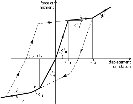
This is a curve frequently employed to model idealised trilinear asymmetric behaviour. An isotropic hardening rule is adopted, and ten parameters need to be defined in order to fully characterise this response curve:

Initial stiffness in positive region (K0+)
The default value is 1000

First branch positive displacement limit (d1+)
The default value is 1

Second branch stiffness in positive region (K1+)
The default value is 50

Second branch positive displacement limit (d2+)
The default value is 5

Third branch stiffness in positive region (K2+)
The default value is 100

Initial stiffness in negative region (K0-)
The default value is 10000

First branch negative displacement limit (d1-)
The default value is -5

Second branch stiffness in negative region (K1-)
The default value is 35

Second branch negative displacement limit (d2-)
The default value is -15

Third branch stiffness in negative region (K2-)
The default value is 100

Notes

1. Stiffness values K0+, K1+, K2+ and K0-, K1-, K2- must be positive. Further, K1 and K2 should always be smaller than K0 in both positive and negative displacement regions.
2. Example. To model the pounding of two adjacent buildings separated by an expansion joint of 20 mm, the following trl_asm curve parameters could be adopted: K0+ = 1e12, d1+ = 0, K1+ = 0, d2+ = 1e10, K2+ = 0, K0- = 1e12, d1- = 0, K1- = 0, d2- = -20, K2- = 1e10. However, the employment of response curve gap_hk is recommended for these cases.
3. Users may refer to the figure in here, for further indications on the cyclic rules employed this response curve. Ultimately, users are always advised to run simple cyclic load analyses (e.g. using a single link element connected to the ground on one end, and then imposing cyclic displacements at its free node) in order to gain a full understanding of this hysteretic relationship, before its employment within more elaborate models.