Load curves
In the Load Curves section, the time-history curve is defined either through direct input of the values of time and load pairs (Create function) or by reading a text file where the load curve is defined (Load function).
Important: The text file of the load curve must be in MS-DOS Windows format (i.e. save the file as ANSI (encoding) using the Notepad).
Usually, static time-history analysis is employed to model simple cyclic tests on specimens, in which case the loading curve is fairly simple and users tend to define it directly within SeismoStruct with the Create option. In the case of dynamic analysis, on the other hand, the applied curve commonly, though not exclusively (e.g. impact/blast analysis), consists of an accelerogram, with data points found in a text file, which is then loaded into the program with the Load option. Nonetheless, any of the two time-history definition options (Create and Load) can be used for both analysis types.
The Analysis Start Time is the time at which the analysis starts, and is always considered as equal to zero, for which reason all time-history curves must feature time entries larger than 0.0. Further, when time-history curves are to be applied to the structure at different time instants (e.g. asynchronous seismic input, two earthquakes hitting the same structure in succession (coincident nodes to be used), etc.), the Delay parameter should be used to define the time at which a particular time-history, being loaded from a text file, starts being applied to the structure. In other words, there is no need for the user to manually change the time-history data points to introduce a time delay, since the program does it automatically.
Whenever there is some uncertainty with regards to the file loading parameters (time column, acceleration column, first line, last line) to be specified, the user can make use of the View Text File facility which permits inspection of the file. After the time-history is loaded, the aforementioned input parameters can still be modified (e.g. if after loading a 5000 lines accelerogram file it is realised that only the first 1000 data points are of interest). The Update View button can be used to visualise in graphic output the resulting changes.
The first line value (equal to 6 by default) essentially specifies the number of lines to be neglected from the beginning of the file. Commonly, accelerogram text files contain introductory header lines, describing their source, characteristics, etc. Evidently, these lines are not to be read by the program. As an example, consider the corrected accelerogram files obtained from the European Strong Motion Database, where a 31 lines header is usually found. For these cases, the first line to be read becomes evidently equal to 32.
The last line parameter (automatically detected by the program) is also needed for those particular cases where the text file contains additional information after the acceleration values. This is a typical behaviour for files coming from a number of strong motion databases whereby velocity and/or displacement time-histories follow their acceleration counterparts. In such cases, it is evidently needed for the last line value to point to the last line of acceleration values.
Accelerograms to be processed in SeismoSignal can feature a maximum of 2^18 data points (i.e. 262144). It is noted, however, that original records featuring an excessive number of data points (e.g. >10000) may lead to slow analyses and, in some cases, system errors, due to the very large memory requirements, for which reason users are advised to crop such large input accelerograms (they typically contain large portions of negligible motion at their start and end) and/or double their time-step (in case an excessively small dt is being employed).
Further, depending on the type of text file format being read, other input file parameters must be defined, as described below.
Single-value per line input text files
To open accelerograms saved in this single-value per line type of format, users must specify one additional input file parameter, i.e. the column in which the acceleration values are to be found.
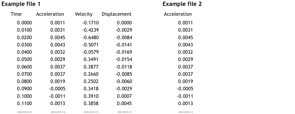
In the case of Example 1 defined above, the Acceleration column would have the value 2 (values in all other columns are ignored by the program), whilst in the case of Example 2, the acceleration column should be defined as 1.
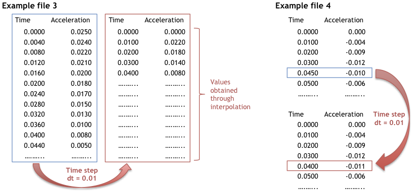
Time & Acceleration values per line input text files
To open accelerograms saved in this Time & Acceleration values per line type of format, users must specify one additional input file parameter (with respect to the previous case), i.e. the column in which the time values are to be found.
Users can find this option useful:
- to load time-histories with a time-step that can then be changed automatically by the program (through interpolation) to the time defined in 'Time Step dt' (see Example 3 below). It can be used in the following cases: (i) the input file features non regularly-spaced time instants, (ii) the input file features a time-step that is too coarse for adequate processing, (iii) the input file features a time-step that is exaggeratedly small, and that will thus unnecessarily delay the analyses or lead to computer memory problems (due to the ensuing very large matrices that are generated by the program);
- to load time-histories defined through non regularly-spaced time steps; the time step that is then adopted by the program is the one defined in 'Time Step dt' (see Example 4 below).
Multiple-value per line input text files
To open accelerograms saved in this Multiple-value per line type of format, users must specify also two additional input file parameters; the Frequency of reading and the initial values skipped. A frequency value of 1 means that all values are read, frequency 2 means that every other value is read, frequency 3 means that one in three values is read (typically used in case of files where values of acceleration, velocity and displacement are given in sequence).
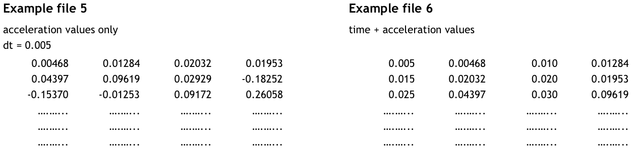
In the case of Example 5 defined above, the frequency to be defined would be 1 (and the initial values skipped should be 0), whilst in the case of Example 6, the frequency value should be 2 (and the initial values skipped should be 1).
ESM Format files
To open accelerograms saved in the ESM format, users do not need to specify any additional input file parameter, since these parameters are automatically detected by the program.
Note: In case that users do not wish to load the whole accelerogram, they might make the proper modifications by changing the values of the First and/or Last line, the Scaled Factor, the Frequency and the Initial Values Skipped. Users are advised to have a deep understanding of the ESM format before making any modification to the above parameters.
SMC Format files
To open accelerograms saved in the SMC format, users do not need to specify any additional input file parameter, since these parameters are automatically detected by the program.
Note: In case that users do not wish to load the whole accelerogram, they might make the proper modifications by changing the values of the First and/or Last line, the Scaled Factor, the Frequency and the Initial Values Skipped. Users are advised to have a deep understanding of the SMC format before making any modification to the above parameters.
PEER NGA Format files
To open accelerograms saved in the PEER NGA format, users do not need to specify any additional input file parameter, since these parameters are automatically detected by the program.
Note: In case that users do not wish to load the whole accelerogram, they might make the proper modifications by changing the values of the First and/or Last line, the Scaled Factor, the Frequency and the Initial Values Skipped. Users are advised to have a deep understanding of the PEER NGA format before making any modification to the above parameters.
Users can also take advantage of the 'Change Units' facility to set the units used by the program as equal to those of the input file.
Once an accelerogram has been defined, the corresponding velocity and displacement time-histories, as obtained through single and double time-integration, respectively, are automatically computed (using the trapezoidal rule) and plotted in the Time Series program window.
Notes
- After loading a time-history curve from a given text file, the latter can be disposed of, since the time-history curve points are saved within the project file itself.
- In order to help users getting started, a set of eight accelerograms, normalised to [g], is provided in the program's installation folder, to where the user is automatically directed whenever he/she presses the Select File button. Users are also referred to online strong-motion databases for access to additional accelerograms.