Analysis Type (Lateral Load Profile or Record Generation)
In SeismoBuild both linear and nonlinear methods are available for the structural assessment. Linear Static and Linear Dynamic procedure may be selected, as well as the two most accurate methods in the assessment practice of existing buildings are employed, that is the nonlinear static pushover analysis and the nonlinear time-history dynamic analysis.
Linear Static Procedure
With the Linear Static Procedure (Lateral Force Method with the EC8 naming conventions) a lateral, pseudo-seismic force distribution with a triangular profile is assumed to approximate the earthquake loading. The forces are applied to a linear elastic structural model, in order to calculate the internal forces and the system displacements.
The different load patterns that will be applied to the structure are defined in this module in two ways:
- The first is by selecting one of the pattern schemes as defined by the Codes, i.e. (i) Basic Combinations, (ii) Eurocode 8, (iii) ASCE 41-23, (iv) NTC-18 (v) KANEPE and (vi) TBDY. By choosing one of these schemes the appropriate load patterns will be selected.
- The second way is to choose individual user-defined load patterns from the corresponding checkboxes. Users may decide about the simultaneous or not application of the lateral incremental loads in the two horizontal directions (Uniaxial or Biaxial load patterns) and the existence or not of Single and/or Double Eccentricity.
Linear Dynamic Procedure
The Linear Dynamic Procedure (Modal Response Spectrum Analysis, according to the EC8 naming conventions) is similar to the LSP, at least as regards the modelling approach. The model is again elastic and there is no stiffness degradation during the analysis. However, the method is somehow more sophisticated, since the profile of the lateral forces is not arbitrary anymore, but rather it is calculated as a combination of the modal contributions of the different modes of vibration of the structure.
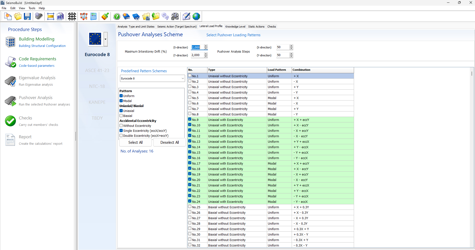
Pushover Analysis
The different load patterns that will be applied to the structure are defined in this module in two ways:
- The first one is by selecting one of the pattern schemes as defined by the Codes, i.e. (i) Basic Combinations, i.e. the uniform and modal patterns without eccentricity in the X and Y directions, (ii) Eurocode 8, (iii) ASCE 41-23, (iv) NTC-18, (v) KANEPE and (vi) TBDY. By choosing one of these schemes the appropriate load patterns will be selected.
- The second way is to choose individual load patterns from the corresponding checkboxes. Users may decide about the vertical distribution of loads (uniform and/or modal patterns), the simultaneous or not application of the lateral incremental loads in the two horizontal directions (Uniaxial or Biaxial load patterns) and the existence or not of Single and/or Double Eccentricity.
The maximum interstorey drift in X and Y direction, as well as the analysis steps in X and Y direction are also defined here.
Dynamic Analysis
Upon selecting this type of the analysis the method of generation of the accelerograms to be used in the analysis need to be specified.
If one of three artificial accelerogram generation methods is selected, the Artificial Record Generation module is displayed. The user may select the number of artificial accelerograms to be generated, the target spectrum settings (minimum and maximum period for matching, and the scaling factor for the defined target spectrum), the record settings (time step and duration), as well as the generation algorithm.
The three methods currently available in SeismoBuild for the simulation of artificial ground motions:
- Synthetic Accelerogram Generation & Adjustment [Hallodorson & Papageorgiou, 2005]
- Artificial Accelerogram Generation [Gasparini & Vanmarcke,1976], which is the default option
- Artificial Accelerogram Generation & Adjustment
The Artificial Accelerogram Generation and Artificial Accelerogram Generation & Adjustment methods are based on the adaptation of a random process to a target spectrum. The adaptation is based on the frequency content using the Fourier Transformation Method, and the adjustment in the second method is done in frequency domain. Only the target spectrum is required for the generation of an accelerogram in both cases.
On the contrary, for the generation of synthetic accelerograms some basic knowledge of the geotectonic environment and the soil conditions relative to the region/site of interest are required. The artificial accelerogram is defined starting from a synthetic one and adapting its frequency content using the Fourier Transformation Method. This method is able to efficiently provide good results, but it has the disadvantage of additional input other than the target spectral shape (earthquake regime, near or far-field, the expected earthquake magnitude, the distance from the source, and the soil conditions).
Instead of selecting one of the three aforementioned artificial accelerogram generation methods, there is the option to load real accelerograms without adjustment.
The display of the RotD100 spectrum is also available.
The ability to employ only the X component or only the Y component of accelerogram, when running dynamic time-history analysis in the Nonlinear Dynamic Procedure is also available in all the above-mentioned methods.