Elastic Response Spectra

Elastic acceleration, velocity and displacement response spectra can be computed and compared in SeismoMatch. The elastic spectra is computed by means of time-integration of the equation of motion of a series of single-degree-of-freedom systems, from which the peak displacement, velocity and acceleration response quantities are then obtained and plotted in period, frequency or displacement vs. amplitude graphs, commonly known as response spectra. In addition, the pseudo-velocity and pseudo-acceleration response values, obtained through multiplication of the displacement response values by ω and ω², respectively, are also given ("ω" stands for angular frequency). Users are referred to the literature [e.g. Clough and Penzien, 1994; Chopra, 1995] for further details on these procedures.

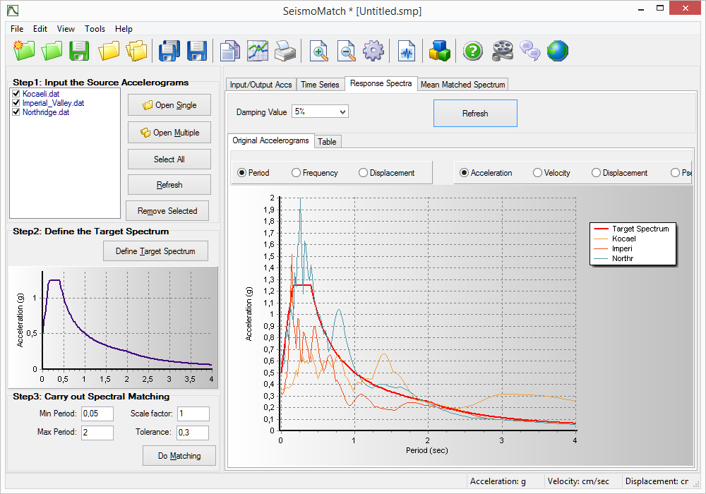
After defining the damping parameter, users need only to click on the Refresh button to initiate the required calculations, noting that these might take some seconds if the computation of elastic spectra for several accelerograms has been requested. Upon completion, the results are automatically shown in the respective modules, where a number of different plotting combinations are made available to the user, including the possibility of changing the parameters being shown on each axis. Moreover, the corresponding spectral values are provided in the 'Displacement', 'Velocity', 'Acceleration', 'Pseudo-Velocity' and 'Pseudo-Acceleration' tables, ready to be selected and copied to other Windows applications, if required. Look in here for further guidance on exporting results.

It is noted that, by default, the damping value shown in this module corresponds to the choice made by the user in the Target Spectrum Definition module, then used in the spectrum matching calculations. Any changes made here to the damping value will thus not affect the target spectrum, nor cause the matching exercise to be re-run, but rather simply allow the visualisation at different levels of damping of the records spectra (hence rendering the comparison between the latter and the target spectrum no longer necessarily meaningful).

Damping
The user has the possibility of changing the level of viscous damping associated to such elastic spectrum, defined here as a percentage of the critical damping value, and usually featuring values ranging from 0 to 5% [e.g Chopra, 1995]. Damping values higher than this limit can also be employed to produce Overdamped spectra.

(Note: the following parameters can be defined/customised in the Program Settings menu)

Numerical integration parameters
Determination of elastic response spectra requires the computation of peak response values of SDOF oscillators with varying periods of vibration that are subjected to the acceleration time-history under consideration. Therefore, linear dynamic analysis needs to be carried out, and a numerical direct integration scheme is employed in order to solve the system of equations of motion [e.g. Clough and Penzien, 1994; Chopra, 1995]. In SeismoMatch, such integration is carried out by means of the Newmark integration scheme [Newmark, 1959].
The Newmark integration scheme requires the definition of two parameters; beta (β) and gamma (γ). Unconditional stability, independent of time-step used, can be obtained for values of β ≥ 0.25 (γ + 0.5)². In addition, if γ = 0.5 is adopted, the integration scheme reduces to the well-known non-dissipative trapezoidal rule, whereby no amplitude numerical damping is introduced, a scenario that is clearly advantageous within the scope of the current application. The default values are therefore β = 0.25 and γ = 0.5.
It is noted, however, that the trapezoidal rule does require the use of relatively small time-steps in order to deliver sufficiently accurate solutions, the reason for which a maximum ratio between the integration time-step and the period of the oscillator being analyzed is imposed (max dt/T = 0.02, by default). As a starting point, the program uses the time-step of the loaded accelerogram as the time-step of the dynamic analysis, and then checks if this does not result to be larger than 2% (or any other threshold value adopted by the user) of the period of the system being analysed. If it is indeed greater, then the algorithm automatically changes the integration time-step so that the maximum dt/T ratio is respected, subdividing, through linear interpolation, the input accelerogram, as required for integration of the equation of motion. It is noted that the maximum dt/T default value (dt/T = 0.02) commonly leads to sufficiently accurate solutions, for which reason users are usually not required to change this value. In any case, if so interested, users need only to carry out a sensitive study in order to determine the largest dt/T value that provides fully precise solutions.

Spectral period range and step
The minimum and maximum periods of interest can be defined by the user, so as to characterise the spectral period range. Usually, for standard structural applications, these correspond to 0.02 and 4.0 seconds, respectively. In addition, the period step value, employed in the computation of the different values that make up the spectra, is also to be defined. The default value if 0.02 seconds. A ductility value and a hardening ratio needs to be defined in other to compute this kind of spectra.